Show code for library loading
# Load necessary libraries
library(psych)
library(GPArotation)
Attaching package: 'GPArotation'The following objects are masked from 'package:psych':
equamax, varimin
Imagine you asked a group of elite athletes to complete a questionnaire containing a set of questions about lifestyle behaviours including hours of sleep, level of protein intake, daily engagement in moderate-to-vigorous physical activity etc.
It would be reasonable to assume that an elite athlete would respond similarly to each of these questions. You’d expect them to have (for example) higher levels of each variable, compared to non-athletes.
It’s also reasonable to suspect that there is an underlying ‘dimension’ to their responses - which we might call ‘athleticism’ or ‘dedication’. This underlying dimension explains how they answer the different questions.
We can’s measure the factor directly, but we can speculate that it exists and causes similar responses on the questions.
Factor analysis is an important statistical method used to describe variability among observed, correlated variables in terms of a potentially lower number of unobserved variables called ‘factors’.
So in the example above, our observed variables are correlated because of an unobserved variable or factor that we could call ‘athleticism’ (or ‘professionalism’, or ‘commitment’…).
Factor analysis aims to find the underlying structure in a set of variables.
It reduces the observed variables into a few unobserved factors for data simplification and to identify groups of related variables.
For example, think about the following variables:
These are different measures, but could reasonably be assumed to represent aspects of one factor, ‘aerobic fitness’.
Factor analysis allows us to reduce several variables into a smaller number of such factors.
Where a factor is unobserved directly, we call it a latent factor, or a latent variable.
For example, we might have a set of questions, each of which is designed to capture some aspect of an underlying factor:
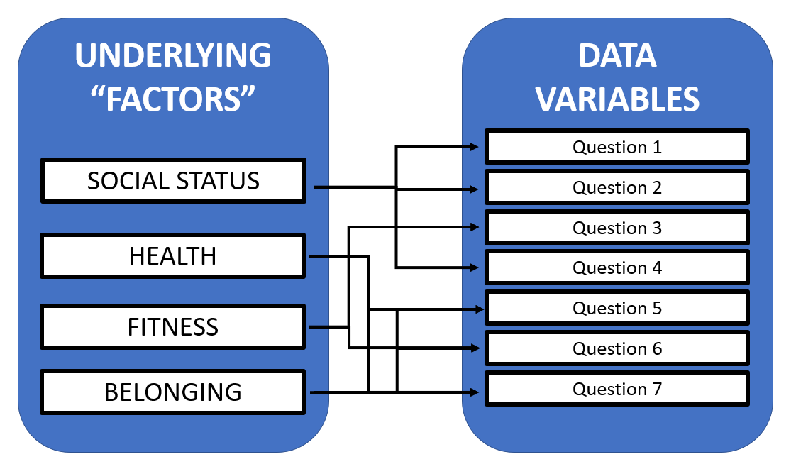
Our series of seven questions actually represent a smaller number (in this case, four) of ‘factors’ or ‘dimensions’.
We can expect responses to each question that is associated with a broader factor to be correlated with other questions that are similarly associated with that factor. This is the basic assumption of factor analysis.
As such, factor analysis is useful for:
Data reduction and simplification: factor analysis reduces a large number of variables into a smaller set of underlying factors, making it easier to analyse and interpret complex data sets.
Identifying underlying structures: factor analysis helps in uncovering the underlying structure or patterns in a set of variables. By doing so, factor analysis can reveal relationships that might not be immediately apparent.
Improving measurement instruments: in fields like psychology and education, factor analysis is often used to develop and refine measurement instruments, such as tests and surveys.
Construct validation: factor analysis is crucial in validating the construct validity of a test. It helps in understanding if the variables grouped together actually represent the theoretical construct (such as intelligence) they are supposed to measure.
Data visualisation: by reducing the dimensionality of data, factor analysis can make it easier to visualise complex datasets.
Handling multicollinearity: you should recall that, in regression models, multicollinearity (high correlation among independent variables) can be problematic. Factor analysis can help in addressing this issue by combining correlated variables into a single factor, which can then be explored within a regression analysis.
EFA is used to uncover the underlying structure of a relatively large set of variables. We use this when we don’t know how many dimensions might underpin our variables, but suspect that there might be some underlying dimensions.
CFA is used to test if measures of a construct are consistent with a researcher’s understanding of the nature of that construct (more theory-driven). We use this when we have a good reason to predict how many factors underpin our data.
For example, if we have deliberately created a questionnaire that has nine questions, and these questions are designed to reflect three underlying factors, we’d conduct CFA to confirm that the questionnaire does so.
These are the correlations between the observed variables and the underlying factors. The ‘loading’ of a variable on a factor lets us identify which factor the variable is most closely associated with. In the example above, if we had three questions that we thought were ‘explained’ by an underlying factor, we’d expect the responses to those questions to load most heavily on that factor.
These measure of how much of the variance of the observed variables a factor explains.
Imagine you have a lot of data about people’s preferences, like in a survey. Each question might relate to different underlying factors, like personality traits. Factor analysis helps you find these hidden factors.
Now, think of eigenvalues in this setting as a way to measure how much of the variation in your data can be explained by each of these hidden factors. When you perform factor analysis, you’re essentially trying to reduce the complexity of your data by finding a few key factors that explain most of the variations in your responses.
The process involves creating a correlation matrix, which is a mathematical representation of how all the different survey questions relate to each other. Eigenvalues are then calculated from this matrix. Each eigenvalue corresponds to a factor, and the size of the eigenvalue indicates how much of the total variation in your data that factor explains.
A larger eigenvalue means that the factor is more significant in explaining the variability in your data. In practice, you often look for factors with the largest eigenvalues, as these are the ones that give you the most information.
This is why, in factor analysis, we often focus on factors with eigenvalues greater than 1, as they are considered to contribute significantly to explaining the variation in the data set.
Communality refers to the amount of variance in each observed variable that can be explained by the factors identified in the model. Essentially, it indicates how well the model captures the information in each variable.
A tool used to help interpret the factors (e.g., Varimax rotation). There are different types of factor rotation that are used, depending on the focus of the analysis.
If you’re interested in following up on these, you might want to explore oblimin rotation as an alternative to varimax.
Factor analysis is complex. In this final section, I’ve given a top-level example of an exploratory factor analysis (EFA). We’ll cover this in more detail during the practical session.
Don’t worry about all the detail; simply try to understand what is going on.
First, we load some libraries that allow factor analysis in R:
# Load necessary libraries
library(psych)
library(GPArotation)
Attaching package: 'GPArotation'The following objects are masked from 'package:psych':
equamax, variminWe create a synthetic dataset. In this case, I’ll create six variables, with two underlying factors.
# Set seed for reproducibility
set.seed(123)

# Generate a synthetic dataset
n <- 200  # number of observations
x1 <- rnorm(n, mean = 50, sd = 10)
x2 <- x1 + rnorm(n, mean = 0, sd = 5)
x3 <- x1 + rnorm(n, mean = 0, sd = 5)
x4 <- rnorm(n, mean = 30, sd = 8)
x5 <- x4 + rnorm(n, mean = 0, sd = 4)
x6 <- x4 + rnorm(n, mean = 0, sd = 4)

data <- data.frame(x1, x2, x3, x4, x5, x6)
The following step performs an exploratory factor analysis on our dataset. In this exploratory factor analysis (EFA) we’re looking explore whether reducing the data to two ‘factors’ is an effective way of reducing our data.
Note: don’t worry about the warning messages that are produced. Just look at the figure.
# Perform Exploratory Factor Analysis
efa_result <- fa(data, nfactors = 2, rotate = "varimax")
Warning in fa.stats(r = r, f = f, phi = phi, n.obs = n.obs, np.obs = np.obs, :
The estimated weights for the factor scores are probably incorrect. Try a
different factor score estimation method.Warning in fac(r = r, nfactors = nfactors, n.obs = n.obs, rotate = rotate, : An
ultra-Heywood case was detected. Examine the results carefullyprint(efa_result)Factor Analysis using method = minres
Call: fa(r = data, nfactors = 2, rotate = "varimax")
Standardized loadings (pattern matrix) based upon correlation matrix
MR1 MR2 h2 u2 com
x1 0.00 1.00 1.00 -0.0017 1
x2 0.04 0.88 0.77 0.2301 1
x3 0.01 0.88 0.78 0.2191 1
x4 1.00 -0.04 1.00 -0.0040 1
x5 0.88 -0.06 0.78 0.2240 1
x6 0.89 -0.02 0.79 0.2090 1
MR1 MR2
SS loadings 2.57 2.56
Proportion Var 0.43 0.43
Cumulative Var 0.43 0.85
Proportion Explained 0.50 0.50
Cumulative Proportion 0.50 1.00
Mean item complexity = 1
Test of the hypothesis that 2 factors are sufficient.
df null model = 15 with the objective function = 6.27 with Chi Square = 1229.41
df of the model are 4 and the objective function was 0.03
The root mean square of the residuals (RMSR) is 0.01
The df corrected root mean square of the residuals is 0.01
The harmonic n.obs is 200 with the empirical chi square 0.34 with prob < 0.99
The total n.obs was 200 with Likelihood Chi Square = 5.49 with prob < 0.24
Tucker Lewis Index of factoring reliability = 0.995
RMSEA index = 0.043 and the 90 % confidence intervals are 0 0.122
BIC = -15.71
Fit based upon off diagonal values = 1fa.diagram(efa_result)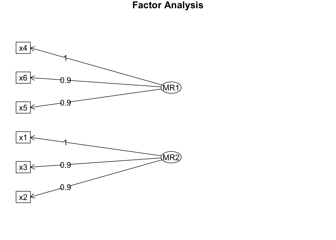
In our analysis, we asked that our six variables be examined in terms of two underlying factors, MR1 and MR2.
As you can see from the printed results, each variable (x1 to x6) has a ‘loading’ associated with each unobserved factor. x4, x5 and x6 appear to load more heavily on MR1, while x1, x2 and x3 load more heavily on `MR2`.
This is a basic example of factor analysis; we’ve reduced responses to six different measures (variables) to a smaller number (two) of ‘underlying’ factors, or dimensions. We’ve also identified which variables are most closely associated with each factor.
In this week’s practical, we’ll work through the steps of a factor analysis in more detail. For now, try to remember that factor analysis attempts to reduce a number of variables to a smaller number of underlying factors, and attempts to evaluate which factor each variable is most closely associated with.
The following reading provides a useful introduction to factor analysis: